ScatterSim:Examples:001Sphere
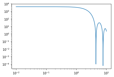
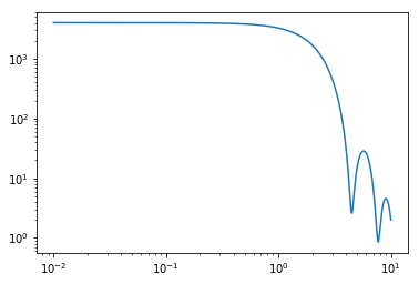
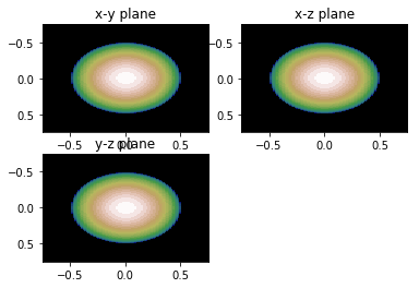
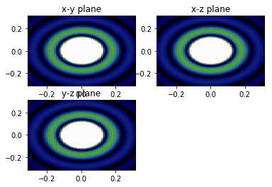
This example shows you how to create a sphere NanoObject and view its 2D form factor, projection, as well as its isotropically averaged form factor. It also shows you how to add polydispersity to your NanoObject. Some code necessary for plotting is deferred at end of document for clarity. Be sure to first copy and paste that code before running the rest.
from ScatterSim.NanoObjects import SphereNanoObject, PolydisperseNanoObject
import numpy as np
import matplotlib.pyplot as plt
%matplotlib inline


# Definining a sphere is simple
pargs_sphere = {'radius' : 1}
sphere = SphereNanoObject(pargs_sphere)

# You can also define a NanoObject with a stochastic parameter
# in this case, we'll make a polydisperse sphere
# The varied parameter will be the radius
pargs_polysphere = dict(radius= 1, sigma_R=.04) # (alternate way of defining dictionaries)
# Just give the object the class you're interested in, and tell it what the parameter it
# is you're varying
# The parameter is assumed to be sampled from a Gaussian distribution of mean 'argname'
# and standard deviation (sigma) 'sigma_R'
polysphere = PolydisperseNanoObject(SphereNanoObject, pargs_polysphere, argname='radius', argstdname='sigma_R')


# Now choose a q domain for the plotting. The units of q will be the inverse of units you supply
# as parameters to the object. For example, we used nanometers, so q will be in inverse nanometers
q = np.linspace(0, 10, 1000)

# finally, calculate
sq_sphere = sphere.form_factor_squared_isotropic(q)
# The polydisperse sphere should take roughly 21 times longer. This is because
# by default it computes the form factors of spheres of radii from 21 points in the distribution
# You can change this, and even change the distribution by reading more into the code
# of NanoObjects.PolydisperseNanoObject
sq_polysphere = polysphere.form_factor_squared_isotropic(q)

# plot using your favorite plotting library
plt.figure(0);
plt.clf()
plt.loglog(q, sq_sphere)
# even with a small polydispersity (4%), polydisperse sphere scattering looks much different
plt.figure(1);
plt.clf()
plt.loglog(q, sq_polysphere)
# For any object, you can compute the form factor or projection. See functions
# above on how to do it.
# P2 means |P|^2 (form factor squared)
qmax = 10
P2_xy, P2_yz, P2_xz = form_factor_slices(sphere, qmax)
rmax = 1.5
V_xy, V_yz, V_xz = sphere.projections(rmax)
# remember this is a 3D Object. We can look at projections of the object in real space
# or slices of the scattering in Fourier (reciprocal) space

show_projections(V_xy, V_yz, V_xz, rmax, 3)
# Showing the form factor

show_qslices(P2_xy, P2_yz, P2_xz, qmax, 2, vmin=0, vmax=6e1)
Plotting code:
def form_factor_slices(smod, qmax):
    ''' Compute the xy, xz, and yz projections.

    '''
    q = np.linspace(-qmax, qmax,100)
    QROWS, QCOLS = np.meshgrid(q,q, indexing="ij")
    Q0 = QROWS*0
    P2_xy = smod.form_factor_squared(np.array([QCOLS, QROWS, Q0]))
    P2_yz = smod.form_factor_squared(np.array([Q0, QCOLS, QROWS]))
    P2_xz = smod.form_factor_squared(np.array([QROWS, QCOLS, Q0]))

    return P2_xy, P2_yz, P2_xz

def show_qslices(F_xy, F_xz, F_yz, length, num=4, **kwargs):
    '''plot the xy, xz, and yz projections with length used from
        projections function, in figure num

        slices go from -2pi/length to +2pi/length
    '''
    extent = 2*np.pi/length*np.array([-1, 1, -1, 1])
    plt.figure(num);plt.clf();
    plt.subplot(2,2,1)
    plt.title("x-y plane")
    plt.imshow(F_xy,extent=extent, **kwargs)
    plt.subplot(2,2,2)
    plt.title("x-z plane")
    plt.imshow(F_xz,extent=extent, **kwargs)
    plt.subplot(2,2,3)
    plt.title("y-z plane")
    plt.imshow(F_yz,extent=extent, **kwargs)


def show_projections(V_xy, V_xz, V_yz, length, num=4):
    '''plot the xy, xz, and yz projections with length used from
        projections function, in figure num
        projections go from -length to +length
    '''
    extent = [-length, length, length, -length]
    plt.figure(num);plt.clf();
    plt.subplot(2,2,1)
    plt.title("x-y plane")
    plt.imshow(V_xy,extent=extent)
    plt.subplot(2,2,2)
    plt.title("x-z plane")
    plt.imshow(V_xz,extent=extent)
    plt.subplot(2,2,3)
    plt.title("y-z plane")
    plt.imshow(V_yz,extent=extent)


