Difference between revisions of "ScatterSim:Examples:001Sphere"
(Created page with "<source lang='python'> from ScatterSim.NanoObjects import SphereNanoObject, PolydisperseNanoObject import numpy as np import matplotlib.pyplot as plt %matplotlib inline # De...") |
|||
| Line 57: | Line 57: | ||
V_xy, V_yz, V_xz = sphere.projections(rmax) | V_xy, V_yz, V_xz = sphere.projections(rmax) | ||
</source> | </source> | ||
| − | + | ||
<source lang='python'> | <source lang='python'> | ||
# remember this is a 3D Object. We can look at projections of the object in real space | # remember this is a 3D Object. We can look at projections of the object in real space | ||
| Line 64: | Line 64: | ||
show_projections(V_xy, V_yz, V_xz, rmax, 3) | show_projections(V_xy, V_yz, V_xz, rmax, 3) | ||
</source> | </source> | ||
| − | [[File:ScatterSimExamples-001- | + | [[File:ScatterSimExamples-001-fig3.png]] |
<source lang='python> | <source lang='python> | ||
# Showing the form factor | # Showing the form factor | ||
| Line 70: | Line 70: | ||
show_qslices(P2_xy, P2_yz, P2_xz, qmax, 2, vmin=0, vmax=6e1) | show_qslices(P2_xy, P2_yz, P2_xz, qmax, 2, vmin=0, vmax=6e1) | ||
</source> | </source> | ||
| + | [[File:ScatterSimExamples-001-fig4.png]] | ||
Revision as of 15:40, 28 March 2017
from ScatterSim.NanoObjects import SphereNanoObject, PolydisperseNanoObject
import numpy as np
import matplotlib.pyplot as plt
%matplotlib inline


# Definining a sphere is simple
pargs_sphere = {'radius' : 1}
sphere = SphereNanoObject(pargs_sphere)

# You can also define a NanoObject with a stochastic parameter
# in this case, we'll make a polydisperse sphere
# The varied parameter will be the radius
pargs_polysphere = dict(radius= 1, sigma_R=.04) # (alternate way of defining dictionaries)
# Just give the object the class you're interested in, and tell it what the parameter it
# is you're varying
# The parameter is assumed to be sampled from a Gaussian distribution of mean 'argname'
# and standard deviation (sigma) 'sigma_R'
polysphere = PolydisperseNanoObject(SphereNanoObject, pargs_polysphere, argname='radius', argstdname='sigma_R')


# Now choose a q domain for the plotting. The units of q will be the inverse of units you supply
# as parameters to the object. For example, we used nanometers, so q will be in inverse nanometers
q = np.linspace(0, 10, 1000)

# finally, calculate
sq_sphere = sphere.form_factor_squared_isotropic(q)
# The polydisperse sphere should take roughly 21 times longer. This is because
# by default it computes the form factors of spheres of radii from 21 points in the distribution
# You can change this, and even change the distribution by reading more into the code
# of NanoObjects.PolydisperseNanoObject
sq_polysphere = polysphere.form_factor_squared_isotropic(q)

# plot using your favorite plotting library
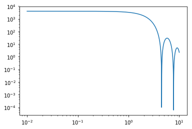
plt.figure(0);
plt.clf()
plt.loglog(q, sq_sphere)
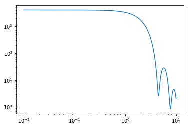
# even with a small polydispersity (4%), polydisperse sphere scattering looks much different
plt.figure(1);
plt.clf()
plt.loglog(q, sq_polysphere)
# For any object, you can compute the form factor or projection. See functions
# above on how to do it.
# P2 means |P|^2 (form factor squared)
qmax = 10
P2_xy, P2_yz, P2_xz = form_factor_slices(sphere, qmax)
rmax = 1.5
V_xy, V_yz, V_xz = sphere.projections(rmax)
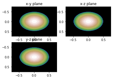
# remember this is a 3D Object. We can look at projections of the object in real space
# or slices of the scattering in Fourier (reciprocal) space

show_projections(V_xy, V_yz, V_xz, rmax, 3)
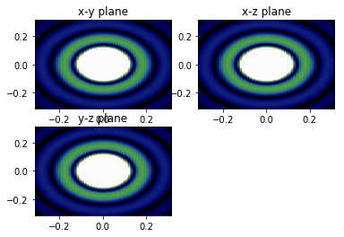
# Showing the form factor

show_qslices(P2_xy, P2_yz, P2_xz, qmax, 2, vmin=0, vmax=6e1)


